Load the file to analyze (see Loading File for Analysis).
If you have done the Input Data process with the FLC tool, the Analysis window should open on the FLC Determination isovalue. The FLC plot should be visible too.
To analysis correctly the FLC, you have to chose the option Final–>Initial.
If not, take the FLC tool and draw a line on the crack. Click on the green arrow ![]() to open the FLC plot. You should have a similare window :
to open the FLC plot. You should have a similare window :
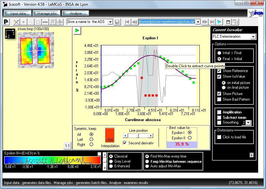
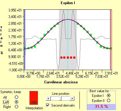
The Line position scroll bar allow to change the section of analysis. The part in grey is represents the crack. The section is represented on the picture by an orange line :
The green and red dots are the values of the isovalue along the line. These dots are interpolated by a sinus curve (in purple on the plot). For a good interpolation, the interpolation coefficient must be higher than 80%. You can see the interpolation coefficient in the gauge at the bottom of the screen :

You can suppress the extreme left and right dots by moving the red and blue verticals lines :
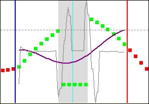
Fitting of the interpolated curve
To increase the interpolation coefficient, you can suppress some bad dots by clicking on it. The red dots are not taken in for the interpolation. The dots above the second derivative curve are usually bad. You can draw the second derivative cure ticking the Second derivative option : 
If you double click on the interpolated curve it will extract the coordinates of the curve :
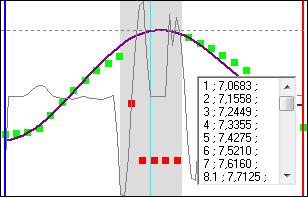
Display of the curve coordinates
You can copy the coordinates and paste it in a spreadsheet program.
If you do not have values in one side, you can copy the opposites values by symmetry with the Symmetry options on the down left corner :

For example, with a left symmetry you will have :
Left symmetry of the curve
You can do the interpolation on the Epsilon I or Epsilon II values by selecting the one you want in the down right frame :
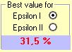
This frame also shows the maximum strain value in percent.